4.5.3. Shape class 3
This shape class describes long crested waves propagating in infinite, constant or varying water depth. Consequently, it may be interpreted as a generalization of Shape 1 and Shape 2. Because the storage and CPU requirements are similar to those specialized classes we may consider to only apply this class for all long crested waves independent of the actual sea floor formulation.
The set of real constants \(k_j\) resemble wave numbers. It follows that the kinematics is periodic in space
where \(\lambda_{\min}\) and \(\lambda_{\max}\) are the shortest and longest wave lengths resolved respectively.
The actual set of shape functions is uniquely defined by the three input parameters \(\Delta k\), \(n\) and \(\hat{n}\).
Note
The fields related to \(j=0\) are uniform in space (DC bias). Non-zero values of \(h_0(t)\) violates mass conservation. The amplitude \(c_0(t)\) and \(\hat{c}_0(t)\) adds a uniform time varying ambient pressure field not influencing the flow field. Consequently, these components will by default be suppressed in the kinematic calculations. However, there is an option in the API for including all DC values provided by the wave generator.
The fields related to \(j=n\) are expected to correspond to the Nyquist frequency of the physical resolution applied in the wave generator. Hence, typical \(n=\lfloor n_{fft}/2 \rfloor\) where \(n_{fft}\) is the physical spatial resolution applied in the wave generator.
4.5.3.1. The sea floor
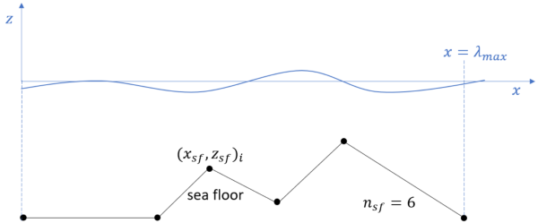
The sea floor \(z_{sf}(x)\) is assumed single valued and is periodic with respect to the \(x\)-location
Hence, the seafloor steepness is finite but may be arbitrary large. In the current version of the API the sea floor is continous and piecewise linear. As illustrated in the figure below, the sea floor is defined by linear interpolation between \(n_{sf}\) offset points \((x_{sf},z_{sf})_i\) for \(i\in\{1,2,\ldots,n_{sf}\}\). The sequence \(x_{sf}(i)\) is monotonic increasing and covering the range \(x_{sf}(i)\in[0, \lambda_{\max}]\)
4.5.3.1.1. Infinite water depth
The infinite depth formulation follows directly by specifying \(n_{sf}=0\) and \(\hat{n}=-1\). Consequently the formulation is equivalent to Shape 1 and there are no spectral amplitudes \(\hat{c}_j(t)\).
4.5.3.1.2. Constant water depth
Constant water depth \(d\) is defined by assigning \(n_{sf}=1\). Hence \(d\equiv -z_{sf}(1)\). The classical shallow water equations (ref Shape 2) are reformulated using exponential terms
Consequently, we only store \(c_j(t)\) in the SWD-file. At the beginning of each new time step we construct \(\hat{c}_j(t)\) using \(c_j(t)\) and the coefficient \(\hat{\gamma}_j\). Because this relation is valid for all time instances the same relations are valid for the temporal derivatives too
This formulation is potential faster and more numerical stable than direct evaluation of the hyperbolic functions.
Hint
In practice \(\hat{n} < n\) because the corresponding neglected high-frequency components do not contribute significantly to any boundary conditions. For the free surface conditions this follows from the property
where \(\zeta_{\max}\) is the maximum wave elevation. Near the sea floor the exponential coefficient \(e^{-2k_j (d + z)}\to 1^-\). Consequently, the contribution to the boundary conditions at the sea floor vanish too, because \(|c_j(t) Z_j(z)|\) vanish for large \(j\).
Due to finite precision arithmetic the following upper limit is recommended
where \(\epsilon_m\) is the machine precision (\(1+\epsilon_m=1\)).
4.5.3.1.3. Varying water depth
Varying water depth (bathymetry) is assumed if \(n_{sf}>1\). In this case also the coefficients \(\hat{c}_j(t)\) needs to be stored in the SWD file.
Hint
For varying water depth, the additional \(\hat{n}\) complex valued coefficients \(\hat{c}_j(t)\) at time \(t\) are expected to be determined in the wave generator by adding zero-flux boundary conditions at \(2\hat{n}\) distributed collocation points on the sea floor.
Due to finite precision arithmetic the following upper limit is recommended
where \(\epsilon_m\) is the machine precision (\(1+\epsilon_m=1\)).
4.5.3.2. Kinematics
Given the definitions above we obtain the following explicit kinematics:
where \(\bar{\nabla}\) denotes gradients with respect to \(\bar{x}\), \(\bar{y}\) and \(\bar{z}\). The particle acceleration is labeled \(\frac{d\bar{\nabla}\phi}{d\bar{t}}\).
The stream function \(\varphi\) is related to the velocity potential \(\phi\). Hence \(\partial \phi/\partial x = \partial \varphi/\partial z\) and \(\partial \phi/\partial z = -\partial \varphi/\partial x\).
4.5.3.3. Implementation notes
Evaluation of costly transcendental functions (\(\cos\), \(\sin\), \(\exp\), …) are almost eliminated by exploiting the following recursive relations
In case the wave generator applies a perturbation theory of order \(q\) we apply the following Taylor expansions above the calm free surface.