This shape class describes a general set of linear Airy waves propagating in infinite or constant water depth \(d\).
Schemes for evaluation of kinematics above \(z=0\) is described below.
\[\phi(x,y,z,t) = \sum_{j=1}^{n} \frac{-g A_j}{\omega_j}Z_j(z)
\sin(\omega_j t - k_{j_x} x - k_{j_y} y + \delta_j) =
\sum_{j=1}^{n} \mathcal{Re} \Bigl\{c_{j}(t)\, E_{j}(x, y)\Bigr\}\, Z_{j}(z)\]
\[\zeta(x,y,t) = \sum_{j=1}^{n} A_j\cos(\omega_j t - k_{j_x} x - k_{j_y} y + \delta_j) =
\sum_{j=1}^{n} \mathcal{Re} \Bigl\{h_{j}(t) \,E_{j}(x, y)\Bigr\}\]
\[E_{j}(x, y) = e^{-i(k_{j_x} x + k_{j_y} y)}, \qquad
Z_{j}(z) = \frac{\cosh k_{j}(z+d)}{\cosh k_{j} d}\]
\[c_{j}(t) = i \frac{g A_j}{\omega_j} e^{i(\omega_j t + \delta_j)}, \qquad
h_{j}(t) = A_j e^{i(\omega_j t + \delta_j)}\]
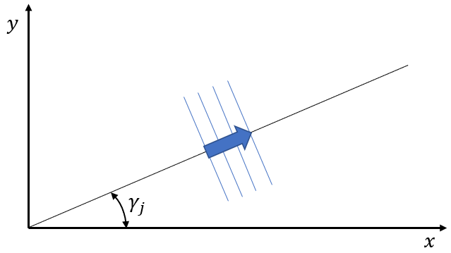
\[\omega_j^2 = k_j g \tanh(k_j d), \quad k_{j_x} = k_j\,\cos\gamma_j,
\quad k_{j_y} = k_j\,\sin\gamma_j, \quad i = \sqrt{-1}\]
4.5.6.1. Kinematics
Given the definitions above we obtain the following explicit kinematics:
\[\phi(\bar{x},\bar{y},\bar{z},\bar{t})= \sum_{j=1}^{n} \mathcal{Re} \Bigl\{c_{j}(t)\, E_{j}(x, y)\Bigr\}\, Z_{j}(z)\]
\[\begin{split}\varphi(\bar{x},\bar{y},\bar{z},\bar{t}) =
\begin{cases}
\sum_{j=1}^n \mathcal{Im} \Bigl\{c_j(t)\, E_{j}(x, y)\Bigr\} \hat{Z}_j(z), & \text{if all $\gamma_j=\gamma_1$},\\
0, & \text{otherwise}
\end{cases}\end{split}\]
\[\frac{\partial\phi}{\partial \bar{t}}(\bar{x},\bar{y},\bar{z},\bar{t}) = \sum_{j=1}^{n}
\mathcal{Re} \Bigl\{\frac{d c_j(t)}{dt}\, E_{j}(x, y)\Bigr\}\, Z_{j}(z)\]
\[\zeta(\bar{x},\bar{y},\bar{t})= \sum_{j=1}^{n}
\mathcal{Re} \Bigl\{h_{j}(t) \,E_{j}(x, y)\Bigr\}\]
\[\frac{\partial\zeta}{\partial \bar{t}}(\bar{x},\bar{y},\bar{t}) = \sum_{j=1}^{n}
\mathcal{Re} \Bigl\{\frac{d h_j(t)}{dt} \,E_{j}(x, y)\Bigr\}\]
\[\frac{\partial\zeta}{\partial \bar{x}}(\bar{x},\bar{y},\bar{t}) = \zeta_x\cos\beta - \zeta_y\sin\beta, \qquad
\frac{\partial\zeta}{\partial \bar{y}}(\bar{x},\bar{y},\bar{t}) = \zeta_x\sin\beta + \zeta_y\cos\beta\]
\[\zeta_x =\sum_{j=1}^{n} k_{j_x} \mathcal{Im} \Bigl\{h_{j}(t) \,E_{j}(x, y)\Bigr\}\]
\[\zeta_y = \sum_{j=1}^{n} k_{j_y} \mathcal{Im} \Bigl\{h_{j}(t) \,E_{j}(x, y)\Bigr\}\]
\[\bar{\nabla}\phi(\bar{x},\bar{y},\bar{z},\bar{t}) =
[\phi_x\cos\beta - \phi_y\sin\beta, \phi_x\sin\beta + \phi_y\cos\beta,\phi_z]^T\]
\[\phi_x = \sum_{j=1}^{n}
k_{j_x}\mathcal{Im} \Bigl\{c_{j}(t)\, E_{j}(x, y)\Bigr\}\, Z_{j}(z)\]
\[\phi_y = \sum_{j=1}^{n}
k_{j_y}\mathcal{Im} \Bigl\{c_{j}(t)\, E_{j}(x, y)\Bigr\}\, Z_{j}(z)\]
\[\phi_z = \sum_{j=1}^{n}
\mathcal{Re} \Bigl\{c_{j}(t)\, E_{j}(x, y)\Bigr\} \, \frac{d Z_{j}(z)}{dz}\]
\[\frac{\partial\bar{\nabla}\phi}{\partial \bar{t}}(\bar{x},\bar{y},\bar{z},\bar{t}) =
[\phi_{xt}\cos\beta - \phi_{yt}\sin\beta, \phi_{xt}\sin\beta + \phi_{yt}\cos\beta,\phi_z]^T\]
\[\phi_{xt} = \sum_{j=1}^{n}
k_{j_x}\mathcal{Im} \Bigl\{\frac{d c_j(t)}{dt}\, E_{j}(x, y)\Bigr\}\, Z_{j}(z)\]
\[\phi_{yt} = \sum_{j=1}^{n}
k_{j_y}\mathcal{Im} \Bigl\{\frac{d c_j(t)}{dt}\, E_{j}(x, y)\Bigr\}\, Z_{j}(z)\]
\[\phi_{zt} = \sum_{j=1}^{n}
\mathcal{Re} \Bigl\{\frac{d c_j(t)}{dt}\, E_{j}(x, y)\Bigr\} \, \frac{d Z_{j}(z)}{dz}\]
\[\frac{d\bar{\nabla}\phi}{d\bar{t}}(\bar{x},\bar{y},\bar{z},\bar{t}) =
\frac{\partial\bar{\nabla}\phi}{\partial \bar{t}} +
\bar{\nabla}\phi \cdot \bar{\nabla}\bar{\nabla}\phi\]
\[\begin{split}\bar{\nabla}\bar{\nabla}\phi (\bar{x},\bar{y},\bar{z},\bar{t}) =
\begin{bmatrix}
\phi_{\bar{x},\bar{x}} & \phi_{\bar{x},\bar{y}} & \phi_{\bar{x},\bar{z}} \\
\phi_{\bar{x},\bar{y}} & \phi_{\bar{y},\bar{y}} & \phi_{\bar{y},\bar{z}} \\
\phi_{\bar{x},\bar{z}} & \phi_{\bar{y},\bar{z}} & \phi_{\bar{z},\bar{z}}
\end{bmatrix}\end{split}\]
\[\phi_{\bar{x},\bar{x}} = \phi_{xx}\cos^2\beta - \phi_{xy}\sin(2\beta) + \phi_{yy}\sin^2\beta\]
\[\phi_{\bar{x},\bar{y}} = \phi_{xy}(\cos^2\beta - \sin^2\beta) + (\phi_{xx} - \phi_{yy})\sin\beta\cos\beta\]
\[\phi_{\bar{x},\bar{z}} = \phi_{xz}\cos\beta - \phi_{yz}\sin\beta\]
\[\phi_{\bar{y},\bar{y}} = \phi_{yy}\cos^2\beta + \phi_{xy}\sin(2\beta) + \phi_{xx}\sin^2\beta\]
\[\phi_{\bar{y},\bar{z}} = \phi_{yz}\cos\beta + \phi_{xz}\sin\beta\]
\[\phi_{\bar{z},\bar{z}} = \phi_{zz} = -\phi_{xx} -\phi_{yy}\]
\[\phi_{xx} = - \sum_{j=1}^{n}
k_{j_x}^2 \mathcal{Re} \Bigl\{c_{j}(t)\, E_{j}(x, y)\Bigr\}\, Z_{j}(z)\]
\[\phi_{xy} = - \sum_{j=1}^{n}
k_{j_x} k_{j_y} \mathcal{Re} \Bigl\{c_{j}(t)\, E_{j}(x, y)\Bigr\}\, Z_{j}(z)\]
\[\phi_{xz} = \sum_{j=1}^{n}
k_{j_x} \mathcal{Im} \Bigl\{c_{j}(t)\, E_{j}(x, y)\Bigr\}\, \frac{d Z_{j}(z)}{dz}\]
\[\phi_{yy} = - \sum_{j=1}^{n}
k_{j_y}^2 \mathcal{Re} \Bigl\{c_{j}(t)\, E_{j}(x, y)\Bigr\}\, Z_{j}(z)\]
\[\phi_{yz} = \sum_{j=1}^{n}
k_{j_y} \mathcal{Im} \Bigl\{c_{j}(t)\, E_{j}(x, y)\Bigr\}\, \frac{d Z_{j}(z)}{dz}\]
\[\phi_{zz} = \sum_{j=1}^{n}
\mathcal{Re} \Bigl\{c_{j}(t)\, E_{j}(x, y)\Bigr\}\, \frac{d^2 Z_{j}(z)}{dz^2}
= -\phi_{xx} - \phi_{yy}\]
\[\frac{\partial^2\zeta}{\partial \bar{x}^2}(\bar{x},\bar{y},\bar{t}) =
\zeta_{xx}\cos^2\beta - \zeta_{xy}\sin(2\beta) + \zeta_{yy}\sin^2\beta\]
\[\frac{\partial^2\zeta}{\partial\bar{x}\partial\bar{y}}(\bar{x},\bar{y},\bar{t}) =
\zeta_{xy}(\cos^2\beta - \sin^2\beta) + (\zeta_{xx} - \zeta_{yy})\sin\beta\cos\beta\]
\[\frac{\partial^2\zeta}{\partial\bar{y}^2}(\bar{x},\bar{y},\bar{t}) =
\zeta_{yy}\cos^2\beta + \zeta_{xy}\sin(2\beta) + \zeta_{xx}\sin^2\beta\]
\[\zeta_{xx} = -\sum_{j=1}^{n}
k_{j_x}^2 \mathcal{Re} \Bigl\{h_{j}(t)\, E_{j}(x, y)\Bigr\}\]
\[\zeta_{xy} = -\sum_{j=1}^{n}
k_{j_x} k_{j_y} \mathcal{Re} \Bigl\{h_{j}(t)\, E_{j}(x, y)\Bigr\}\]
\[\zeta_{yy} = -\sum_{j=1}^{n}
k_{j_y}^2 \mathcal{Re} \Bigl\{h_{j}(t)\, E_{j}(x, y)\Bigr\}\]
\[p = -\rho\frac{\partial\phi}{\partial \bar{t}}
-\frac{1}{2}\rho\bar{\nabla}\phi\cdot\bar{\nabla}\phi
-\rho g \bar{z}\]
where \(\bar{\nabla}\) denotes gradients with respect to
\(\bar{x}\), \(\bar{y}\) and \(\bar{z}\).
\(\mathcal{Re}\{\alpha\}\) and \(\mathcal{Im}\{\alpha\}\) denote the real and imaginary part of a
complex number \(\alpha\).
The particle acceleration is labeled \(\frac{d\bar{\nabla}\phi}{d\bar{t}}\).
The stream function \(\varphi\) is only relevant for long crested waves and is
related to the velocity potential \(\phi\).
Hence \(\partial \phi/\partial x = \partial \varphi/\partial z\)
and \(\partial \phi/\partial z = -\partial \varphi/\partial x\).
Note that for the stream function evaluation we apply the function
\[\hat{Z}_j(z) = \frac{\sinh k_j(z+d)}{\cosh k_j d}\]